Lewis Carroll once wrote, “If you don’t know where you are going, any road will get you there.” Watts H. Humphrey, the American software engineer countered with “If you don’t know where you are, a map won’t help.” These two quotes remind us about the two essential ingredients of a healthy, continuously evolving process: direction and decisiveness. For a successful global S&OP process, direction and decisiveness are crucial.
We had recently remodeled demand planning process at Hollister and our destination was simple. It was to achieve the following:
- Provide an interchange of thought between Sales, Marketing, Finance, and Operations
- Create meaningful reporting for demand planners and end users
- Focus on risk/opportunity for the company
Demand Planning and Global S&OP Process
Hollister Incorporated employs a global S&OP process divided into three geographical areas – North America, which I manage, is one of those areas. Each geographical area completes tasks on a similar schedule.
Demand Planning has the first six workdays of the monthly S&OP process to report KPIs, revise baseline and/or event forecasts, and review results with key internal partners. Demand Planning finalizes the demand plan, and hands it over to Supply Planning on day seven. Supply Planning creates a replenishment plan by the ninth workday. A pre-S&OP meeting by global region occurs on the tenth workday. The company demands a firm time schedule and fully engaged participants in order to deliver the report on day twelve to our executive S&OP meeting. The director of Global Operations, to whom the Demand Planning and Supply Planning teams report, presents key supply/demand imbalances and any required or volunteered action plans to our executives.
Also, the demand planning function at Hollister separates forecasts into two succinct categories – operational and budgetary forecasts. Operational forecasts consist of combining the revenue and sample forecasts. Revenue forecasts apply to products sold to customers. Sample forecasts apply to products provided to customers and sales representatives free of charge for demonstration and education. Budgetary forecasts consist of an annual plan and a modification of the annual plan during the middle of our fiscal year. My focus will be on the operational forecasting process.
Demand Plan Process: An Overview
The overall steps in the demand planning process remain the same: report KPIs, revise the demand plan, and review the revised plan with internal team members impacted by the changes. These steps occur during the first seven workdays of the month. I suspect this is a common practice in many companies.
For Hollister, I made some minor adjustments to KPI reporting. We still calculate forecast accuracy (error) using MAPE. However, now I include forecast accuracy tolerances by product segments meaningful to the end users including Marketing, Finance, and Sales. In the past, forecast accuracy was tracked to show improvement only. Now, not only do they show improvement but whether the accuracy for the current period is within acceptable parameters specific to a category of products.
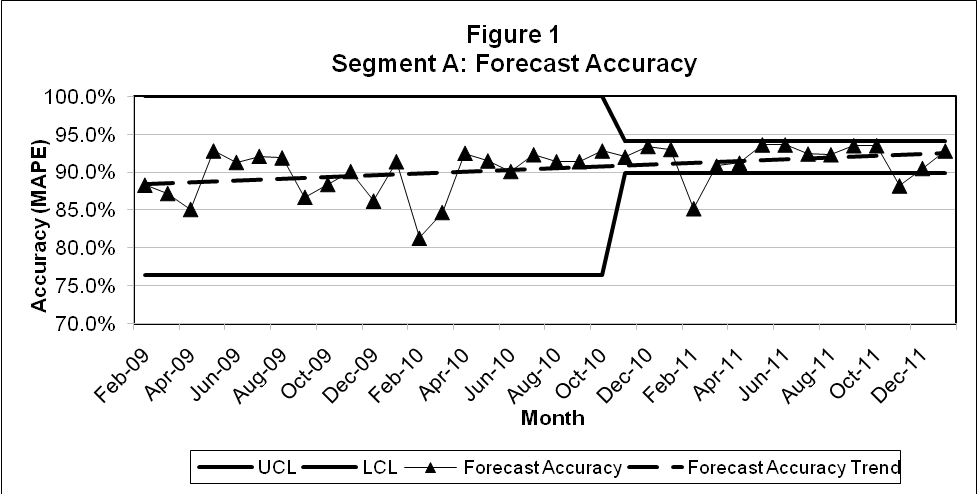
As shown in Figure 1, the solid lines represent the upper and lower control limits. These are calculated with a varying range of standard deviations, depending on the business. Every point on the graph shows the forecast accuracy for that period, monthly in this case. The dashed line denotes the current trend.
Reports should be transparent, actionable, and tell the story. Transparency is simple. All Demand Planning reports are available for review by any team member either on a shared hard drive or via our intranet. The above report accomplishes the remaining two requirements. The report details the history of this particular business, the overall improvement not only in forecast accuracy but also in forecasting stability. Forecast accuracy has been improving from around 88% in August 2008 to 92% by June 2011. Not only has accuracy been improving, it also has been consistently getting better. The upper and lower control limits have narrowed to the range of 90% to 94%. This enabled the production team to rely more on forecasts than on their consumption data, to reduce their safety stock level, and to make improvements on their Just-in-Time standards. Also, the report demands action by the forecaster to continually improve results and to identify and repair causes of outliers like the one evidenced in February 2011 (see Figure 1).
Basic reporting is formatted similarly to the S&OP and financial reporting. The sample report later in this article displays this discipline. This maintains familiarity in reporting for the same audience, namely executive leadership. Reporting, including Demand Planning, adopts the corporate standard usually established by Finance.
Revising the demand plan requires considerable attention to avoid pitfalls and to build credibility. Four steps encompass the demand plan revision stage of Hollister’s demand planning process:
- Cleansing and managing historical data
- Maintaining a cyclical SKU-L review
- Managing forecast exceptions
- Reviewing event forecasts
A Good Cleansing
The first step in revising the demand plan is data cleansing. The “garbage in garbage out” theory in computer programming applies here as well. Forecast models, especially regression and exponential smoothing, exhibit sensitivity to outliers or unique events spanning over one or several periods. Neutralizing the outlier or event is the science part. Understanding what caused the outlier or whether the event is extremely important is the art part of demand planning. The demand planner can only adjust outlier(s) or system parameters if the cause is known and understood. For example, a plant explosion in the hometown of a major customer needed our wound care products for numerous burn victims. This was a one-time event because it does not happen every day. The entire purchase is removed from the data. In another example, initial orders by new customers are used not only to stock their shelves but also to cover their demand between order cycles and safety stock. Going forward, they will only replace what they sell. Based on our experience, we expect the future demand of such a customer be approximately 40% of the initial order. Therefore, we remove 60% of the initial demand data. Of course, timing of when sales will begin and when ramping up of demand will occur also requires some adjustments.
A Cyclical Approach
The second step is developing and maintaining a cyclical SKU review based on volume and variability. I like to think of my SKUs as children; I have 3,200 of them running around needing their own special attention—some more than others. Therefore, SKUs with high volumes and variability are reviewed monthly or semi-monthly (especially new product launches or focus products). Focus products often contain event forecasts. Medium volume products with high variability and vice versa are reviewed on a monthly basis. Products with lower volume and higher variability are reviewed less frequently; that is, quarterly. (See Figure 2)
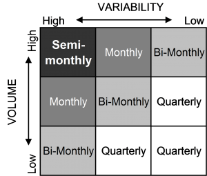
We use this model for reviews based on item variability.
Figure 2: Forecast Review Based on Volume and Variability
I determine each SKU’s coefficient of variability on an annual basis. The same is true for classifying a SKU’s volume. A-volume SKUs comprise 80% of the company volume. B-volume SKUs make up the next 15% of volume. And C-volume SKUs are the last 5%. However, I calculate a SKU as high, medium, or low volume within each marketing or sales manager’s area of responsibility. In some businesses, total unit volume does not equal the unit volume of one SKU in another business. Focus products qualify automatically for semi-monthly review.
Manage The Exceptions
The next to last step in the process is managing exceptions. This is accomplished using system alerts from APO-DP (SAP’s Advanced Planning Optimizer for Demand Planning) and reporting out of SAP’s Enterprise Data Warehouse (or Business Warehouse or Intelligence) application. Two classifications of alerts or reporting exist—responsive and reactive. Responsive alerts and reporting provides advance warning of what might happen with potential outliers and forecast accuracy challenges. Whereas, reactive alerts and reporting detail what happened. The goal of the process is to be 100% proactive and rarely, if ever, reactive. Time spent in reaction mode is time lost on learning the business and improving the process. Again, I cannot reiterate how important it is to understand what caused a miss in accuracy or an unforeseen outlier.
Review The Event
The last step in the process involves the event review meeting with Sales, Marketing, Finance, and Operations. The level of detail varies depending on how stable an event’s demand is and how knowledgeable the Sales and Marketing team is about the forecasting process. I will comment on this later. If variability is high, then we review at the SKU-Location level. If the event stabilizes, then we review at an appropriate aggregate level according to our company product hierarchy. Forecast accuracy and bias are calculated for each event as well. Again, the reporting must be actionable and tell a story.
| Table 1: Accuracy of a New Product Launch | ||||||
| Product Line J. Smith | January-11 | February-11 | March-11 | April-11 | May-11 | June-11 |
| New Product Launch | 78.2% | 69.6% | 58.6% | 53.5% | 91.7% | 98.6% |
Table 1 reveals the story of forecast accuracy of a particular new product launch, which improved only after suffering some performance anxiety. This forecast required investigating why accuracy plummeted after the January 2011 launch. Two causes were identified. One, key customers did not readily adopt the new product similar to its predecessor. Two, customers were unsure how to properly use the new product. As you can see, Demand Planning in partnership with Sales and Manufacturing answered the challenge through forecast adjustments and enhanced customer training.
Monthly Demand Planning S&OP Meeting
The monthly demand planning meeting typically involves representatives from Sales, Marketing, Operations, and Finance. The purpose of the meeting is threefold: Identify supply constraint impacts on event forecasts and timing, close the gap between the demand and supply, and then approve the demand plan. Notice we identify supply constraints only. Hollister, Incorporated develops an unconstrained forecast.
The meeting agenda is divided into three parts: present causes behind any KPI out of tolerance limit, discuss key events with biggest impact on business, and then approve the demand plan. Not only are the causes of KPIs performing outside tolerances presented, but solutions developed or actions to be taken are presented as well.
Regarding the discussion of events, documented observations and any action taken are shared with Operations. This provides Operations (sometimes Finance) an opportunity to ask questions or to share any constraints with Sales and Marketing. Oftentimes, the constraint is known and already responded to.
| Table 2 Demand Plan of Region A: 2011 | |||||||
| Current | Prev. Demand Plan | AOP | Mid-Year | ||||
| Demand Plan | June 2011 | DP vs. Previous | 2011 AOP | DP vs. AOP | 2011 Mid-Year | DP vs. MY | |
| Category A | 1,597,000 | 1,592,400 | 0.3% | 1,624,000 | -1.7% | 1,594,900 | 0.1% |
| Category B | 2,555,800 | 2,533,600 | 0.9% | 2,579,500 | -0.9% | 2,547,400 | 0.3% |
| Category C | 1,060,500 | 1,063,100 | -0.2% | 1,089,500 | -2.7% | 1,055,500 | 0.5% |
| Category D | 1,607,000 | 1,597,200 | 0.6% | 1,643,200 | -2.2% | 1,592,900 | 0.9% |
| Category E | 9,100 | 9,200 | -1.1% | 10,000 | -9.0% | 9,200 | -1.1% |
| Total Product Line 1 | 6,829,400 | 6,795,500 | 0.5% | 6,946,200 | -1.7% | 6,799,900 | 0.4% |
| Category F | 6,400 | 5,900 | 8.5% | 5,500 | 16.4% | 6,000 | 6.7% |
| Category G | 8,700 | 8,700 | 0.0% | 9,000 | -3.3% | 8,600 | 1.2% |
| Category H | 278,900 | 248,200 | 12.4% | 272,800 | 2.2% | 279,600 | -0.3% |
| Total Product Line 2 | 294,000 | 262,800 | 11.9% | 287,300 | 2.3% | 294,200 | -0.1% |
| Category I | 100,800 | 100,900 | -0.1% | 92,300 | 9.2% | 94,700 | 6.4% |
| Category J | 384,000 | 389,200 | -1.3% | 346,700 | 10.8% | 366,100 | 4.9% |
| Category K | 4,900 | 4,900 | 0.0% | 4,000 | 22.5% | 4,500 | 8.9% |
| Category L | 90,400 | 90,200 | 0.2% | 72,500 | 24.7% | 92,400 | -2.2% |
| Category M | 1,400 | 1,400 | 0.0% | 1,200 | 16.7% | 1,500 | -6.7% |
| Total Product Line 3 | 581,500 | 586,600 | -0.9% | 516,700 | 12.5% | 559,200 | 4.0% |
| Category N | 113,000 | 113,000 | 0.0% | 124,400 | -9.2% | 118,900 | -5.0% |
| Category O | 28,600 | 27,900 | 2.5% | 25,800 | 10.9% | 27,400 | 4.4% |
| Category P | 29,300 | 30,500 | -3.9% | 38,600 | -24.1% | 31,800 | -7.9% |
| Total Product Line 4 | 170,900 | 171,400 | -0.3% | 188,800 | -9.5% | 178,100 | -4.0% |
| Total – Region A | 7,875,800 | 7,816,300 | 0.8% | 7,939,000 | -0.8% | 7,831,400 | 0.6% |
The current demand plan is compared against the previous demand plan, the annual plan (AOP), and the mid-year adjustment. At times, it is necessary to share causes behind any larger-than-normal increases or decreases. For example, Category H, as shown in Table 2, would require explanation regarding an increase of 12.4% over the previous month’s demand plan. In this particular case, Sales won a new contract with a high volume customer.
What About The Rest Of The Month?
With regard to performing the above tasks, the balance of the month is spent monitoring performance (including going over the response-based alerts and reporting), managing forecasts on an as-needed basis (adding new product forecasts, adding or adjusting new events, or adjusting existing baseline), and mentoring internal customers on demand planning process and procedures. Every interaction offers the opportunity to reinforce basic principles, such as forecasts should reflect expected sales not a method of inventory management. As alluded to earlier, the training and understanding of internal partners is part of the process.
This article originally appeared in the Journal of Business Forecasting, Spring 2012 issue. To receive the Journal of Business Forecasting become an IBF member today.