
As I have written about before in a previous article, Forecasting Materials Usage At An Electric Utilities Company, forecasting efforts for an electric utility company are imperative.
Forecasting is an essential part of our demand management tactics and without forecasting diligence and a proactive approach to managing inventory, our organization is exposed to the risk of not delivering electricity to customers.
Forecasting helps us investigate the future to make decisions on what quantities of materials we need to proactively order. This exercise helps us maintain appropriate inventory levels so that our organization can fulfill demand while at the same time maintain a lean inventory that does not commit unnecessary capital.
But what happens when our forecasting efforts are ineffective? What happens when we under-estimate, or over-estimate what we will need in the future? It’s not hard to imagine the consequences of the forecasted demand being off from actual demand. We will risk stocking out on materials, or we will have excessive inventory sitting idly.
Recognizing Error
I respond to errors in the forecast in a couple of ways. The first step is to recognize the error. Was the forecast over or under actual demand, and by how much? The magnitude of the error is of more importance to me. If the forecast was only slightly off, I will not pay it much attention.
We understand that forecasting will generally be different from what occurs, to some extent, so being close is a win. If the forecast is off by a large amount, then it’s time to act.
Calculating Size of the Error
What is a large amount? That will vary from forecast to forecast. For example, a widget’s forecasted consumption may have an absolute deviation (absolute error) of 1,000 units in a month. Said differently, the forecasted quantity could have been 10,000 units while actual consumption was only 9,000 units – we over-forecasted by 1,000 units. Being off by 1,000 units may sound like a lot but, if we take the absolute percentage error formula
Absolute Value((Actual – Forecasted)/Actual X 100))
Absolute Value(9,000 -10,000)/9,000) X 100 = 11%
we get a mere 11 percent. With the absolute percentage error, the lower the number the better. The absolute percentage error metric provides a deeper understanding of how close the forecast was.
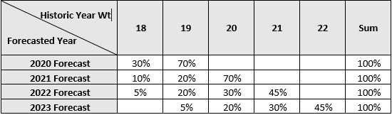
If I am using a weighted forecasting model, in which I take the average demand of the same month over different years e.g., January 2018, January 2019, January 2020, and January 2021, I can then assign a different weight to each year. I typically assign a higher weight to more recent years because the recent past will often – but not always – be a better predictor of the near term.
The below table exhibits how I typically assign weights to years in a weighted forecast.
After assigning the above weights in a forecast model for a particular widget, I found that the forecast was a fair amount off in one month. The below graph helps to illustrate how the forecast in February 2022 was off from the actual.
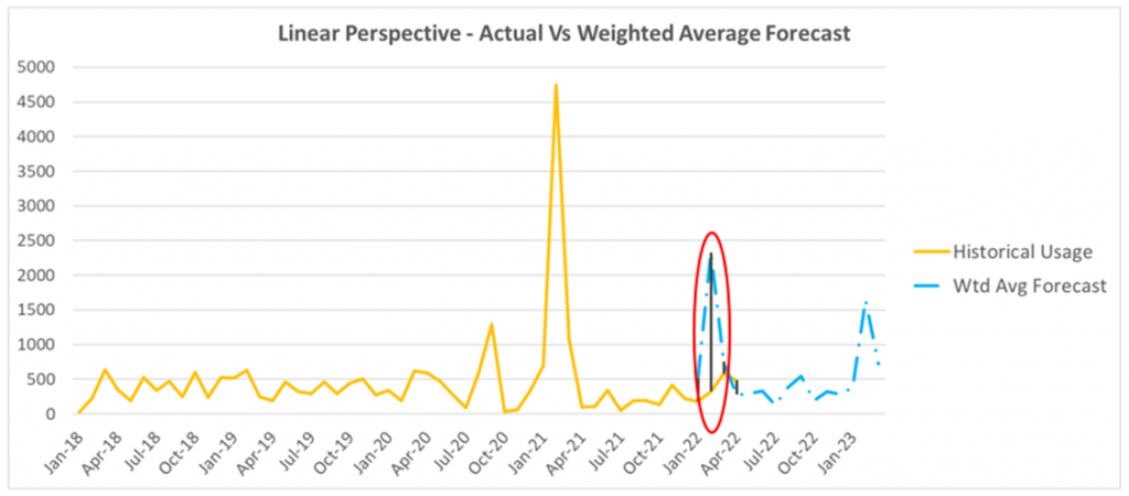
The red circle around the February 2022’s data shows the vertical line between the turquois blue (actual consumption) and the light blue dashed line (Weighted Average Forecast) to illustrate how off the forecast was from actual consumption.
In February 2022, our actual consumption for this widget was 324 units, but the forecast was 2,328 Units. This was an absolute deviation (aka absolute error) of 2,004 units. The absolute percentage error was 619 percent. Here is where the next step of the action comes in.
After noticing this significant deviation, I considered the usage from the years 2020 and 2021. As you can see from the graph above, the consumption reached dramatically higher points in these years than in 2018 and 2019; this is one of the instances where the recent past is not a better predictor of the near future.
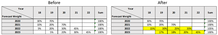
It is safe to say that the months of consumption in 2020 and 2021 may result in an overstated forecast if we give more deference to these years. To address this concern, I adjusted the weights from my pervious table. I reduced the weights from the years 2021 and 2020 both by 10 percent and added 10 percent to both 2019 and 2020.
The new weights are reflected in the below tables. I made these adjustments for 2022’s Weighted Average forecast and made similar adjustments to the year 2023’s Weighted Average Forecast.
After adjusting the weights, the forecasted quantity for February 2023 was reduced from 1,638 units to 1,235 units and appears to be more in line with previous Februarys.
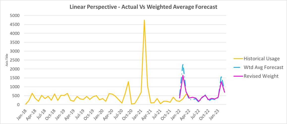
The adjustments I made to the weights in the model project a forecast for the rest of 2022 and for the first quarter of 2023 that I feel quite comfortable with. February 2023’s new forecasted consumption of 1,235 is still rather high. The average monthly consumption over the past four years is only 462 units. Though it is unlikely that 1,235 units will need to be in our available inventory in February 2023, I would much rather have our organization be in the position where we are somewhat overstocked than substantially understocked.
The strategy of whether to carry a heavy inventory or lean inventory will vary from widget to widget. Some widgets will have far less of a risk appetite than others. For these items, the approach of over-estimating, and the consequence of excessive inventory, is one that we want to live with as opposed to the risk of stocking out. The aforementioned scenario shows us how connected forecast modeling is to an inventory strategy – a topic that certainly deserves more explanation in another article.
How I React When The Error is Large
These are the steps in the process I use to react to forecasts when there is a significant deviation from actual demand. A summary of the process is as follows.
Step 1: Review the item’s forecasted demand to actual demand and identify where there are big variances. Use metrics such as the absolute error (absolute deviation) and absolute percentage error to validate that there was a deviation that deserves attention.
Step 2: Review the historical demand and then adjust the calculations in the forecast as necessary. In the case of the weighted average forecast, one can easily make weight adjustments to the years, or time periods, in which historic demand may be understating or overstating the forecasting model.
Another possible step may include adjusting the historic demand data sample. For example, if the years 2020 and 2021 demonstrate a clear downward trend of decreased demand from 2018 and 2019, it may make sense to completely remove the years 2018 and 2019 from the forecast’s data sample. The new sample would include only the past 24 months of demand instead of the past 48 months.
There is nearly an endless number of ways in which you could change the approach to forecasting when there is a significant difference in forecasted demand from actual demand.
Perhaps an even simpler approach is to change the forecasting model all together. Instead of applying a Weighted Average forecast, one could use a Simple Linear Regression model, or Exponential Smoothing model. Whichever the forecasting methodology you use, the same basic steps of reviewing the differences in the forecast against the actual will be necessary to determine your next course of action.
IBF’s Supply Chain Planning Boot Camp returns to Las Vegas from August 10-12. Learn the fundamentals and best practices across the supply-demand chain and how leading companies balance supply and demand, from the demand plan to the master scheduling process. More information here.