At my former company, Bendix Commercial Vehicle Systems, an Ohio-based manufacturer of brakes and safety systems, I was asked to come up with a list of seasonal items across multiple levels of product hierarchy.
The product hierarchy was part → plant → device code → main family, and was spread across several plants, focusing exclusively on the aftermarket portion of the business. The project developed into a means of identifying seasonality via multiple indicators and approaches, culminating in the use of a statistical forecasting model for comparison against moving average models. Below is a summary of the project complete with the process steps and outputs. The primary tools used were Excel and the R forecasting package.
Starting With Time Series Decomposition
To accomplish this task, I went back to some basic yet powerful statistical concepts, beginning with time series decomposition. In time series decomposition, seasonality can be separated from noise and trend (at least in theory). I ended up identifying seasonality in 2 ways – the first was with Excel, using a median demand value over each year compared to each month’s demand patterns. Excel doesn’t have a decomposition feature, so I performed this manually.
In this case, if the output (what I called “indices”) were the same or close for over 75% of the year, I considered it to be seasonal. The reason why I allowed values that were ‘close’ as well as the same was to account for any rounding or fluctuation in decimals as decimals were not recorded to every decimal place.
Having the ability towards the end of the project to program in R, I used the default time series decomposition function in this package to identify seasonality as well. R seemed to confuse (or fail to distinguish seasonality) from noise in the time series tested. This I attribute to natural fluctuations in demand levels from year to year. Given my earlier analysis in Excel, I was fairly confident that seasonality existed in the dataset, so I started looking at other models that could confirm or deny this. I eventually utilized Holt-Winters filtering to filter the time series which indeed confirmed the existence of seasonality.
Holt-Winters Filtering
The results of the Holt-Winters filtering were quite different than standard time series decomposition. Because of the noise in the time series, the default time series decomposition in R did not adequately identify seasonality – but Holt-Winters filtering did (see Figure 1).
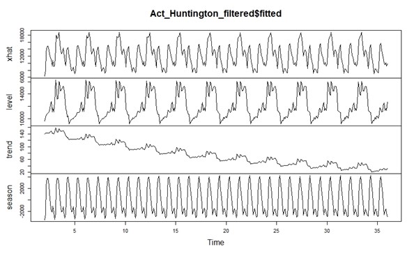
Figure 1. Identifying seasonality with Holt-Winters Filtering
Filtering is also a powerful tool for optimizing a time series. Holt-Winters filtering also allowed for the determination of coefficients across various periods. The goal of this was to look for coefficients that repeated over time at the same (or nearly the same) periodicity with roughly the same value. This would support my theory that seasonality was present in the dataset as coefficients should roughly change at the same interval if seasonality were present – values could change but the pattern of repeating was a strong indication of seasonality. Given this was a test for seasonality, the specific values were not extremely important at this stage but rather the pattern of coefficients and the intervals. See Figure 2 for the fitted plot and for a plot of the coefficients.
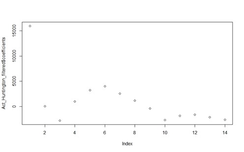
Figure 2. A plot of the coefficients using Holt-Winters Filtering
Another important aspect of this project was to perform “what if” analysis, i.e., what seasonal demand might look via a simulation. In most instances, a uniform distribution was used, employing a minimum and maximum based on historical demand. In Excel and R, this was performed with a randomized uniform distribution.
At some combinations at higher levels of product hierarchy, discrete distributions were used but later analysis revealed little to no seasonality at lower levels. This led me to use uniform distribution for the combinations, which show seasonal behavior.
Results show that demand does follow a seasonal pattern with a roughly consistent cycle over the 36 months of demand history. The simulations were run first based on an interval for 1 year and then for an interval over the entire 3 years of demand history with little to no change in results.
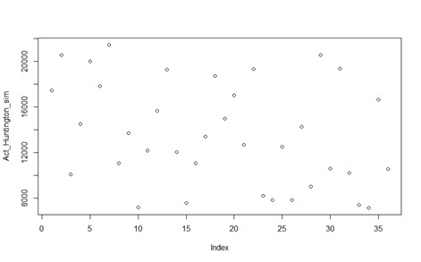
Figure 3. Demand showing a seasonal pattern.
Given this project was done as part of a demand planning and forecasting team, the natural progression was to determine how to deliver a better forecast for seasonal items. Utilizing averages will often lead to over smoothing on seasonal items unless the seasonality occurs on the same cycle or line as the average. Rather than attempt to tune the moving average, I utilized a 6-month moving average for comparison purposes and my baseline.
Harnessing the power of R forecasting package, I was able to perform a triple exponential smoothing forecast. The forecast is based on the original time series with 36 points which results in a forecast for 36 months. The package fits the forecast to the time series and provides the resulting coefficients for each of the periods as well. These coefficients allowed for forecast comparison on demand and the six month moving average as well. See below (Figure 4) for comparisons between demand (actuals) and triple exponential smoothing and 6 month moving average.
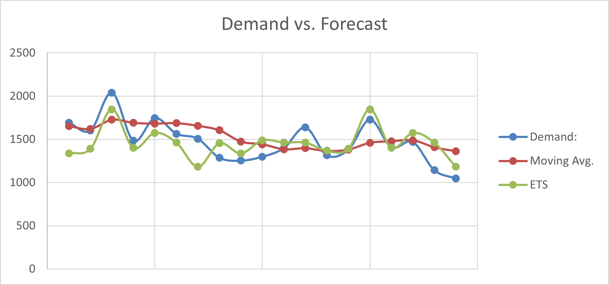
Figure 4. Forecast vs. actual demand
At the end of this project, 6 out of 30 product groups showed seasonality which is approximately thirty percent of the entire product portfolio. Statistical and quantitative analysis allows for comparison of time series and determination of seasonal coefficients and simulation. But just as important are consideration of non–quantitative factors as well. These may include customer, markets and perhaps other external factors such as structural shifts or product advancements.
Hopefully this will provide a simple yet useful means to identify seasonality and ultimately assist in developing a robust forecast.